Monitored Quantum Circuits

Authors

[Ali G. Moghaddam]

Abstract

Introduction to monitored quantum circuits

A monitored quantum circuit (MQC) refers to a digital quantum computer or simply quantum circuit that allows for both quantum measurement and quantum gates (unitary operations) during the computation. While in a standard quantum circuit, typically the input state is transformed into a final state only through a sequence of quantum gates, and the measurement (readout) is carried out in the final stage, a MQC includes also measurements at intermediate times in the evolution of the circuit.

From a merely quantum computational perspective the mid-circuit measurements can be exploited for the sake of observing and potentially correcting the quantum state before the final readout. On the other hand and from a fundamental point of view, it has been found recently that these quantum circuits with random unitaries and local measurements can offer a new interesting platform for investigating quantum many-body physics and collective phenomena far from equilibrium. Long-standing theoretical questions such as thermalization in closed quantum systems, quantum chaos, and entanglement dynamics all seem to show up in the monitored random quantum circuits. Also, recent experimental progress in building digital quantum simulators has made random quantum circuits a more natural playground in the noisy intermediate-scale quantum (NISQ) era and without the need for true quantum advantage.

The flagship phenomenon in these systems, which is under intense study by various groups worldwide, is what is known as the measurement-induced entanglement phase transition. In brief, while the application of two- and multi-qubit unitary gates yields further entanglement, measurement destroys entanglement and their interplay leads to a critical behavior. The two-side of criticality correspond to distinct phases with volume-law and area-law entanglement, at small and large rates of measurements, respectively. We have been working on this timely topic since late 2022 and as part of our study, I have developed a versatile and efficient Python code to simulate MQCs. In what follows I will first explain the foundations of ranadom monitored quantum circuits and then review the structure of the code and finally describe main ideas and algorithms used in the code implementation.

Quantum circuits and discrete-time quantum trajectories

A schematic of ranadom monitored quantum circuits is shown in Fig. 1 below with horizontal direction indicating the spatial direction of the qubits in a one-dimentional chain and vertical direction showing the time evolution.

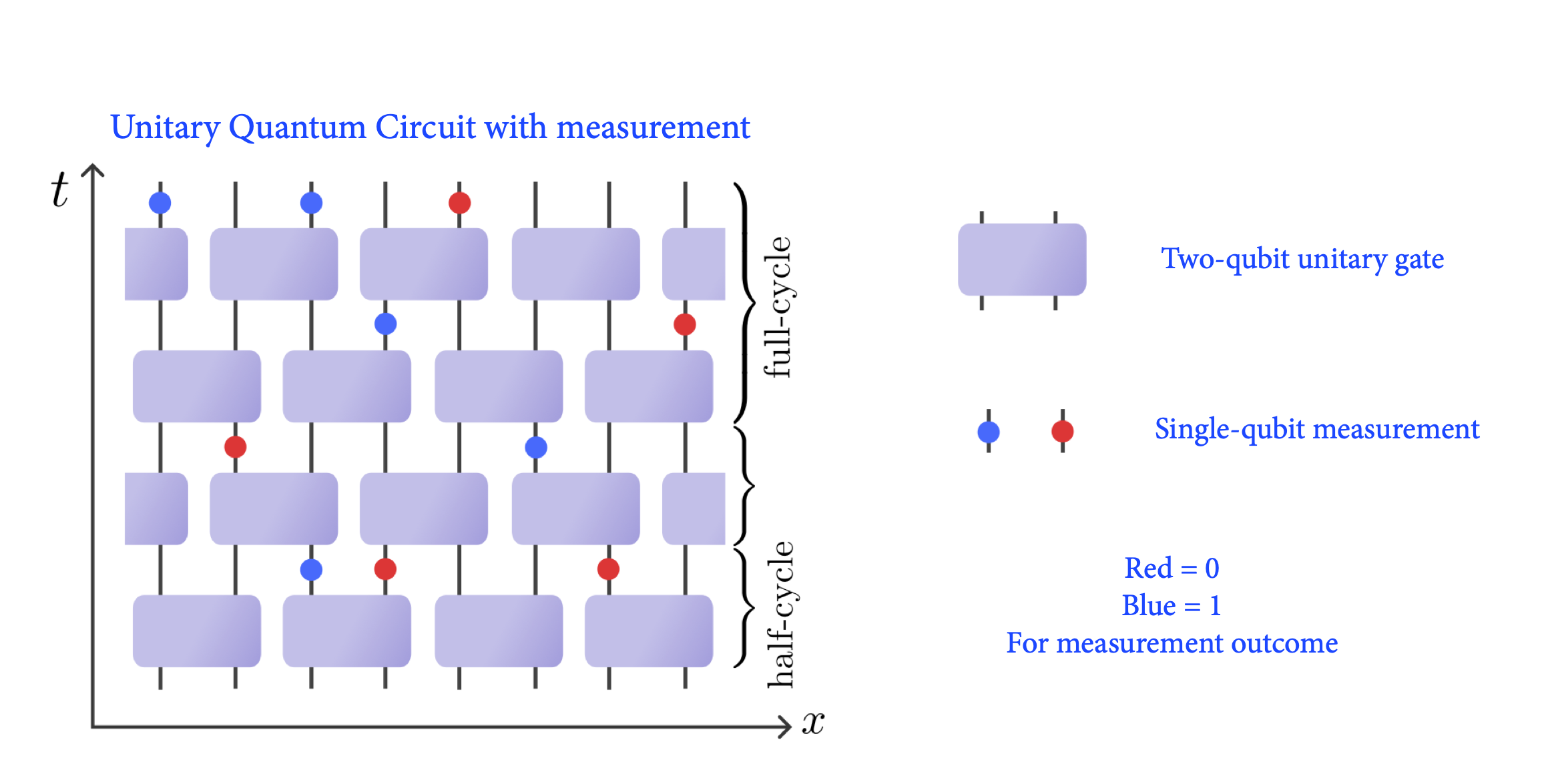
Fig. 1 Schematic monitored quantum circuit At each discrete time step, a set of two-qubit random unitaries are applied followed by a set of single-qubit measurements of randomly chosen sites. Gathering the history of each speial set of maesurement outcomes corresponds to a special quantum trajectory of the circuit. Assuming we have measured $M$ qubits during the time evolution, there will be $2^M$ different quantum trajectories.

It is easy to understood that applying certain unitaries can generate entangled states from unentangled ones. For instance, considering two qubits in either of states \(|01\rangle\) or \(|10\rangle\) by applying the two-qubit unitary operator

we get entangled states \(\cos \alpha|01\rangle -\sin \alpha|10\rangle\) and \(\sin \alpha|01\rangle+ \cos \alpha|10\rangle\), respectively. For \(\alpha=\pi/4\) these two states will be maximally entangled states (singlet and \(S=0\) triplet states, respectively). This idea can be exploited to design well known quantum circuits to generate on-demand highly-entangled states by successive application of
two-qubit unitaries to a multi-qubit system shown.

Before going to the details of how a quantum circuit operates, we should introduce the useful notation of tensors for presenting manybody states. A general manybody state of \(2N\) \(n\)-bit chain can be written as